Hypothesis Testing - One Way Analysis of Variance (ANOVA) with F-Test

This article describes how to perform a one-way ANOVA with F-test.

To learn about statistical functions in MAQL, see our Documentation.

Background

In Hypothesis Testing - One Sample T-Tests and Z-Tests, we examined comparisons of a single sample mean with the population mean. For situations in which three or more sample means are compared with each other, the ANOVA test can be used to measure statistically significant differences among those means and, in turn, among the means for their populations.

The size of a difference that is statistically significant depends on the sample sizes and the amount of certainty desired in the testing. In our significance tests, we use p-values (levels of statistical significance).

For example, a company's marketing team may want to answer, "Does the day of the week have an impact on the number of clicks?" To frame the question in other terms, we wish to measure whether there is any difference between the number of clicks on different days of the week.

The first step of any hypothesis testing is to convert the question into null and alternative hypotheses:

• null hypothesis (H 0 ): x? Mon = x? Tue = x? Wed = x? Thu = x? Fri = x? Sat = x? Sun (where x? is the average number of clicks in a given day of the week). If the average number of clicks on each day of the week is consistent, the day of the week does not have an impact.
• alternative hypothesis (H 1 ): At least one of the mean values does not equal the others.

To perform this test, we must calculate the F-test statistical value and compare it with the critical value from the F-distribution table, based on the chosen significance level or p-value (usually 0.05) and the degrees of freedom.

Computing ANOVA Table

An ANOVA table comprises the following components:

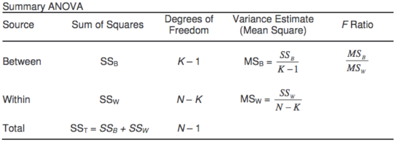
Our goal is to calculate the value of F Ratio in the last column as the final result of computing the values in all of the other columns. Let's review what these table values mean and how we can calculate them in MAQL.

Column 1 - Sum of Squares

SS B = ∑n(x? i -μ) 2 , is the Sum of Squares (deviations) between the group means and the grand mean, where x?i is the group mean and μ represents the grand mean.

Avg Clicks(Mon)

The following MAQL metric computes the average number of clicks for the specified day of the week:

SELECT AVG( Clicks ) WHERE  Day of Week (Mon-Sun) (Date) =Mon

We calculate this metric for each day of the week. These are our group means (x?i).

Avg Clicks(ALL)

The following MAQL calculates the average clicks across all days of the week. This value is our grand mean (μ).

SELECT AVG( Clicks ) BY ALL OTHER

Count(Mon)

The following metric calculates the count of clicks for Monday:

SELECT COUNT( Date(Date) ,  Records of Website ) WHERE  Day of Week (Mon-Sun) (Date) =Mon

We calculate this metric for each day of the week to get the number of records in each group. In our example, the unique identifier for clicks is the Date attribute.

Dev(B,Mon)

(The B above stands for "Between")

SELECT ( Avg Clicks(Mon)  -  Avg Clicks(ALL) ) BY ALL OTHER

This metric gives us the deviation between the groups and the grand mean (x?i-μ). We calculate this for each day of the week.

SSB

Finally, we add n*(x?i-μ) for all the groups to get the value for SSB.

SELECT ((POWER( Dev(B,Mon) ,2) Count(Mon) ) + ((POWER( Dev(B,Tue) ,2) Count(Tue) ) + ((POWER(Dev(B,Wed) ,2)* Count(Wed) ) ...

SST

SS T = ∑(x i -μ) 2 is the Sum of Squares of all the observations from the grand mean (μ), regardless of which group produced them.

SELECT SUM(POWER((SELECT (SUM( Clicks )- Avg Clicks(ALL) ) BY  Date (Date) ),2))

Note how we used the BY  Date(Date)  clause to compute the difference between each observation and the grand mean. In our example, Date is the unique identifier for Clicks.

SSW

SS W = SS T - SS B , is the Sum of Squares within the groups. It is also called Error Sum of Squares and can be calculated by subtracting Sum of Squares between the groups from total Sum of Squares.

SELECT  SST  -  SSB 

Column 2 - Degrees of Freedom

K-1 measures the degrees of freedom between groups, where K is number of groups. In this example, the value is 7 because we are analyzing days of the week.

N-K measures within degrees of freedom, where N is total number of records.

Count(N)

SELECT COUNT( Date(Date) ,  Records of Website )

Column 3 - Mean Square

MS B = SS B / K-1 is the Mean Sum of Squares between the groups. It is calculated by dividing the Sum of Squares between the groups by the between-group degrees of freedom.

MSB

SELECT  SSB / ( K -1)

MS W = SS W / N-K is the Mean Sum of Squares within the group. It is calculated by dividing the Sum of Squares within the groups by the within-group degrees of freedom.

MSW

SELECT  SSW / ( Count(N)  -  K )

Column 4 - F Ratio

F Ratio = MS B / MS W

SELECT  MSB / MSW 

After we have calculated the F-value, we can compare it to the critical value using an F-distribution table and then evaluate the significance of the analysis.

Evaluating Significance

F-Distribution Table

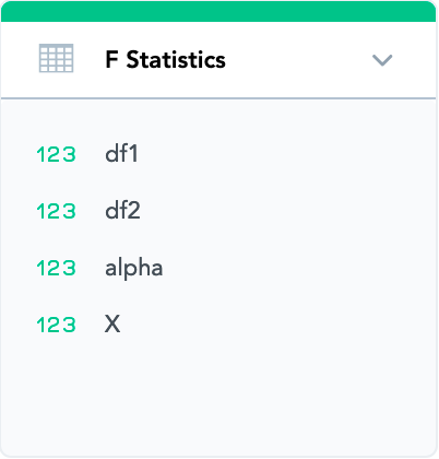
The first step is to upload a table of F-distribution critical values, which you can find in any statistical textbook. Download an example table of F-statistic values in the attached file.
The example table has 4 columns:

• df1 - Between-group degrees of freedom
• df2 - Within-group degrees of freedom
• alpha - Significance level that we desire in our analysis (usually 0.05, 0.01, 0.005)
• X - This column contains the critical value of F-statistic. We compare the F Ratio metric calculated above with this value using the other three columns as lookup values

Fact Dataset in LDM

We create a fact dataset in our logical data model, as shown below, to store these values:

Note that all the four columns are stored as facts.

Upload F-Distribution Data

After you have created the dataset in your logical data model, build a simple ETL graph to upload the data in the file to your project.

Calculate Metrics

After the values have been uploaded to the project, we can use the following metrics to evaluate whether our analysis is significant.

df1(Clicks)

SELECT CASE WHEN ( K -1) > 150 THEN 1000, WHEN ( K -1) > 90 THEN 120, WHEN ( K -1) > 50 THEN 60,WHEN ( K -1) > 35 THEN 40, WHEN ( K -1) > 29 THEN 30 ELSE ( K -1) END

df2(Clicks)

SELECT CASE WHEN (COUNT(N)-K) > 150 THEN 1000, WHEN (COUNT(N)-K) > 90 THEN 120, WHEN(COUNT(N)-K) > 50 THEN 60,WHEN (COUNT(N)-K) > 35 THEN 40, WHEN (COUNT(N)-K) > 29 THEN 30 ELSE (COUNT(N)-K) END

X(Clicks)

SELECT (SELECT SUM( X ) WHERE  df1 = df1(Clicks)  AND  df2 = df2(Clicks)  AND  alpha = Sig Level ) BY ALL OTHER

The Sig Level variable is used to depict significance level, which is usually 0.05 or 0.01.

• If the F Ratio metric is larger than this X value, our analysis is significant.
• If the analysis is valid, we can reject the null hypothesis. In our example, day of the week does have an impact on the number of clicks.