This article describes forecasting techniques that use simple and weighted moving average models for a time series. It also describes how to use a mean absolute deviation approach to determine which of these models yields a more accurate prediction.
Background
The moving average is a very common time series forecasting technique. It is useful when you want to analyze a variable (for example, sales, seminar attendees, returns, accounts, and so on) across several consecutive periods, particularly if no other data is available with which to predict the value of the next period. It is often preferable to use historical data to forecast future values rather than simple estimates.
Moving averages compensate for short-term fluctuations and highlight longer-term trends or cycles. Essentially, moving averages predict the value of the next period by averaging the value of n prior periods.
Simple Moving Average (SMA)
The simple moving average is the average of the values over the last n periods. The number of periods that you should analyze in a moving average forecast depends on the type of movement in which you are interested.
In the formula below, the preceding n values for D are used to calculate the forecasted value F for period t+1.
Ft+1 =(Dt + Dt-1 + - - - + Dt-n+1)/n |
where:
- D is the actual value
- F is the forecasted value.
Weighted Moving Average (WMA)
Sometimes, values from more recent months are more influential as predictors of the value for the coming month, so the model should give them more weight. This type of model is known as a weighted moving average. The weights you use can be arbitrary as long as the sum of weights equals 1:
Ft+1 = w1Dt + w2Dt-1 + - - - + wnDt-n+1 |
Scenario
Suppose a pharmaceutical company wants to predict the demand for their most popular drug to ensure that they have enough inventory on hand for orders in the coming month. To help the company formulate an accurate prediction, the Demand Planning manager analyzes a 3-month moving average, as demand may fluctuate significantly over a quarter.
First, you calculate the predicted value using both SMA and WMA techniques. Then, you set up the model and evaluate which technique yields the more accurate forecast.
Demand(SMA)
SELECT ((SELECT Demand(Sum) FOR PREVIOUS(Month/Year (Demand Date),1)) + (SELECT Demand(Sum) FOR PREVIOUS(Month/Year (Demand Date),2)) + (SELECT Demand(Sum) FOR PREVIOUS(Month/Year (Demand Date),3)))/3
Note that you used a FOR PREVIOUS clause to sum demand from the last three periods. After summing the demand value for the last three periods, you can divide the sum by 3 to calculate the average.
Demand(WMA)
To calculate demand using WMA, you give a weight of 3 to the most recent period, a weight of 2 to the next most recent period, and a weight of 1 to the next most recent period. Note that the ratio for these is 50%: 33%: 17%, which satisfies the requirement that the sum of weights equal 1.
SELECT (0.5*(SELECT Demand(Sum) FOR PREVIOUS( Month/Year (Demand Date) ,1))) + (0.33*(SELECT Demand(Sum) FOR PREVIOUS( Month/Year (Demand Date) ,2))) + (0.17*(SELECT Demand(Sum) FOR PREVIOUS( Month/Year (Demand Date) ,3)))
Slicing these metrics by Month/Year yields the following view:
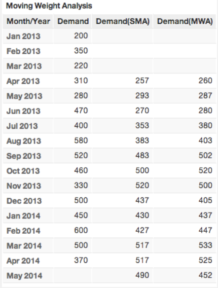
Assuming that the current month is April 2014, you get two values for demand in May 2014: one SMA, and one MWA. Now let's see which of these two values is more accurate.
Determining the Accuracy of a Moving Average Model
Calculating the Mean Absolute Deviation (MAD)
Typically, the quality of a forecasting model is measured by its margin of error between actual and predicted results, and a common measurement of forecast accuracy is mean absolute deviation (MAD). For each forecasted value in the series, you calculate the absolute value of the difference between the actual and forecasted values (the deviation). Then, you average those absolute deviations to calculate MAD.
MAD can help us to decide how many periods to average, the weight to assign to each period, or both. The model with the lowest MAD value is typically our best choice. Let's calculate MAD for the two models:
Deviation(SMA)
SELECT ABS( Demand(SMA) - Demand(Sum) )
Deviation(WMA)
SELECT ABS( Demand(WMA) - Demand(Sum) )
The following table shows the MAD scores for the two models.
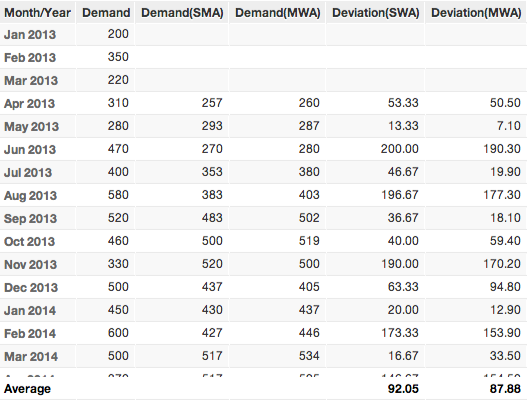
Of the two models, the MAD for MWA (Average for Deviation(MWA)= 87.88) is smaller, so it is more accurate than the SMA model.
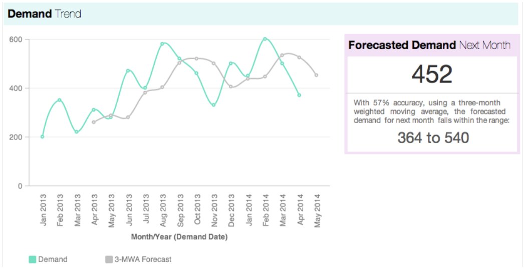
Visualizing the Predicted Value
Generally, a forecast value should also include an accuracy range (high and low). Therefore, in addition to showing the forecast values on a line chart, you should also create a headline report that shows the accuracy percentage.
Control Limits for a Range of MADs
Usually, forecast errors are normally distributed (note that in this example, we're ignoring auto-correlation). Normal distribution results in the following relationship between MAD and the standard deviation of the distribution of error:
1 MAD is approximately 0.8 standard deviations.
This allows us to establish statistical control limits for a range of MADs:
| Number of MADs | Accuracy |
| +/- 1 | 57% |
| +/- 2 | 88.9% |
| +/- 3 | 98.3% |
| +/- 4 | 99.9% |
These limits produce a range of values for the forecast. For example, the forecast value for next month fits the following parameters:
- Ft+1 - 1*MAD and Ft+1 + 1* MAD with 57% accuracy
- Ft+1 - 2*MAD and Ft+1 + 2* MAD with 88.9% accuracy
- . . . and so on.
So, you can say that using a 3-month Weighted Moving Average, the forecast demand for May 2014 = 452+/- 87.88 (276 to 627) with 57% accuracy.
MAD(MWA)
SELECT AVG((SELECT Deviation(MWA) BY Month/Year (Demand Date) )) BY ALL OTHER
Lower Range
SELECT (SELECT Demand(WMA) WHERE Month/Year (Demand Date) = THIS + 1 ) - ( MAD(MWA) )
Upper Range
SELECT (SELECT Demand(WMA) WHERE Month/Year (Demand Date) = THIS + 1 ) + ( MAD(MWA) )