
This article shows how to use MAQL to analyze time-lagged correlations and R2 values between two time series.
To learn about statistical functions in MAQL, see our Documentation.
Background
In the business world the dependence of a variable Y (the dependent variable) on another variable X (the explanatory variable) is rarely instantaneous. Often, Y responds to X after a certain lapse of time. Such a lapse of time is called a lag.
When you are using X values from prior periods to explain the current Y, you should use lagged correlation. Without it, you may fail to detect much of the explanatory power of X.
For example, suppose you want to understand the impact of TV ads on the sales of a product. In that case it would make sense to use a lag of a week or two on the marketing spend and then correlate it with sales. It would not make sense to analyze the spend and sales data as soon as the ad is broadcast because some time must elapse before you can reasonably expect to see an increase in sales.
Scenario
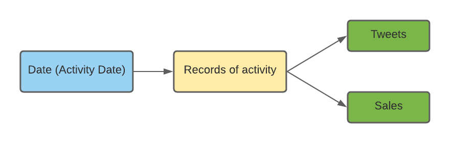
Suppose that you want to analyze the impact of a Twitter campaign on sales. In your model, the Twitter and sales data are joined by the same date (ActivityDate) as shown below.
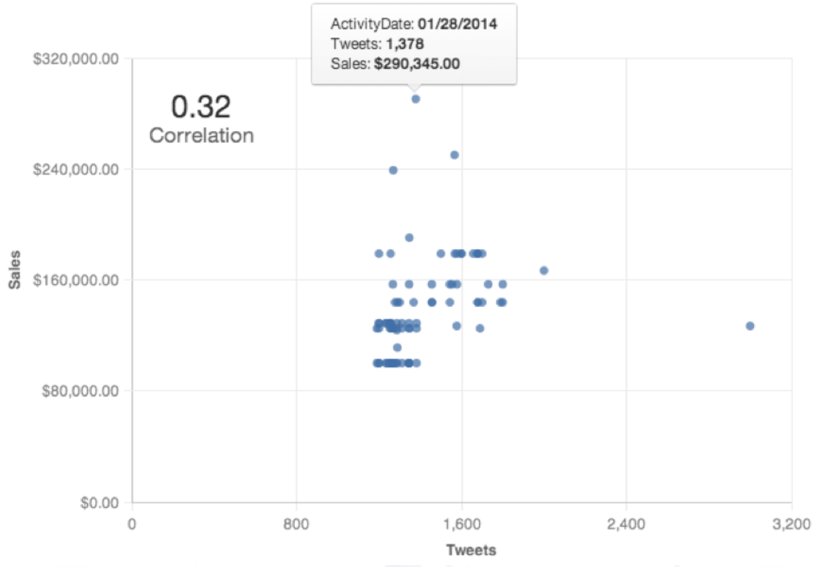
Now if you calculate the correlation between Tweets and Sales and create a scatter plot, you probably wouldn't find a significant correlation (see below):
Metric 1 - Tweets vs Sales (Correl)
The following metric computes the Pearson correlation value. You can use it to create a headline report on top of a scatter plot.
In the figure, notice that the correlation value shows no significant relationship between Tweets and Sales. This is probably because it is unlikely that customers would buy a product immediately after participating in a Tweet campaign. To compensate, in Metric 3 below, you add a 3-day lag to the metric and then recalculate.
The length of time (lag) that should elapse before you see a significant correlation between a campaign and sales probably depends on the type of product or ad campaign in question (among other factors). In the case of vacation packages or furniture purchases, for example, you might expect lags to be measured in months rather than days. For fast-food purchases or discounted merchandise, lags of a few days are more likely.
SELECT CORREL( Tweets , Sales )
Metric 2 - Tweets Lag vs Sales (Correl)
The following metric uses the FOR PREVIOUS clause to generate a lag. You can also specify week, month, and year in a similar way to create a lagged variable. Because you want to see a lag of three days, you specify 3 as a second parameter in the FOR PREVIOUS clause. This metric can be used to create a headline report.
You can use the following metric to create a scatter plot between the lagged number of Tweets variable and the dependent Sales variable.
SELECT CORREL((SELECT SUM( Tweets ) BY Date (ActivityDate) FOR PREVIOUS( Date (ActivityDate) , 3)), (SELECT SUM( Sales ) BY Date (ActivityDate) ))
Metric 3 - Tweets 3 Day Lag
Note that this metric is identical to the first part of Metric 2 above (Correl function).
(SELECT SUM( Tweets ) BY Date (ActivityDate) FOR PREVIOUS( Date (ActivityDate) , 3)
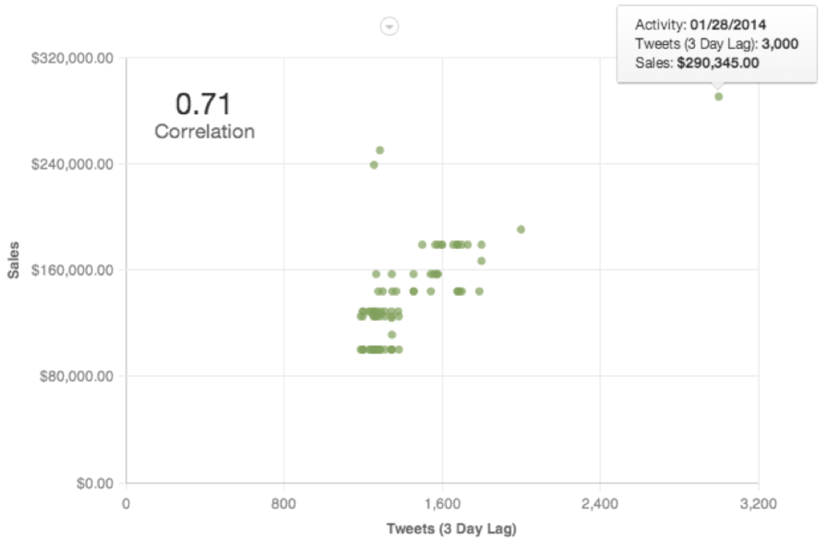
Now the scatter plot between the lagged variable and Sales shows a positive correlation and a correlation change from 0.32 to 0.71. This means that a 3-day lag in Tweets explains the variation in Sales much better than Tweets with no lag.
Coefficient of Determination (R2) with Lagged Variables
After you have calculated a lagged correlation, you can easily calculate how much of the variation in Y is explained by X by squaring the lagged correlation. This is equivalent to the R2 value used to explain regression models.
Coefficient of Determination = Power(Tweets Lag vs. Sales (Correl), 2) |
In this case, the Coefficient of Determination = 0.49 which means that 49% of the variation in Sales can be explained by using the 3-day lag in Tweets.