
This article introduces the metrics for assembling simple linear regression lines and the underlying constants, using the least squares method. You can extend these metrics to deliver analyses such as trending, forecasting, risk exposure, and other types of predictive reporting.
To learn about statistical functions in MAQL, see our Documentation.
Background
Prerequisites
The MAQL calculation requires use of Pearson Correlation (r), which is described in Covariance and Correlation and R-Squared.
Linear Regression
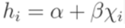
Full regression analysis is used to define a relationship between a dependent variable (y) and explanatory variables (X1, ..., Xp). For tutorial purposes, this simple linear regression attempts to model the relationship between a dependent variable (y) and a single explanatory variable (x) using a regression coefficient (β) and a constant (α) in a linear equation. For each explanatory value xi, this simple model generates an estimate value for yi. This estimate is denoted as hi and is dependent upon only xi, β, and α with the following linear relationship:
This simple linear regression equation is sometimes referred to as a "line of best fit."
Least Squares Approach
The above model attempts to measure the estimated value. The actual difference between the linear model above and the actual dependent yi value can be represented by an error term (εi):

The least squares approach attempts to minimize the sum of the square of the above error terms (ε12+...+εn2). The following five summary statistics support the calculations for the least squares approach:
- Pearson Correlation (r)
- The mean of the explanatory variable (X?)
- The mean of the dependent variable (Y?)
- The standard deviation of the explanatory variable s x
- The standard deviation of the dependent variable s y
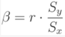
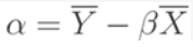
The result yields the following two equalities for β and α:
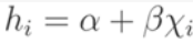
The above metrics enable us to solve for our linear regression equation h:
Scenario
Let's assume the same scenario as the insurance company in the topic Covariance and Correlation and R-Squared.
After we have generated Metric 6: Pearson Correlation (r) defined in the above topic, you can immediately calculate metrics for β, α and our linear estimate hi.
Metric 8 - Beta Regression Coefficient
First, we calculate β using Pearson Correlation (r), the standard deviation of x (Number) and the standard deviation of y (Value):
SELECT ((SELECT Pearson Correlation (r))*(SELECT (SELECT STDEV(Value))/(SELECT STDEV(Number)))) BY ALL OTHER
The BY ALL OTHER clause is used to prevent the amount from being sliced by anything present in the report.
Metric 9 - Alpha Constant
Then, we are able to calculate α using β from above, the mean of x, and the mean of y:
SELECT (Avg Claim Value (Mean Y ) - (Beta * Avg Claim Number (Mean X))) BY ALL OTHER
The two mean metrics are carried over from the topic Covariance and Correlation and R-Squared.
Metric 10 - hi Linear Regression Estimate
We can now calculate our linear regression estimate using α, β, and the x value (Number).
SELECT ( Alpha + ( Beta * (SELECT MEDIAN(Number))))
The MEDIAN function is used in case there are multiple instances of the same x (Number) in your sample. As the x values in your chart are the same, MAX and MIN functions could be used interchangeably.
Application
Add the linear regression line to your graph
The resulting hi linear regression estimate metric can be added to the What tab in a report along with your SUM( Value ) metric to show your "line of best fit":
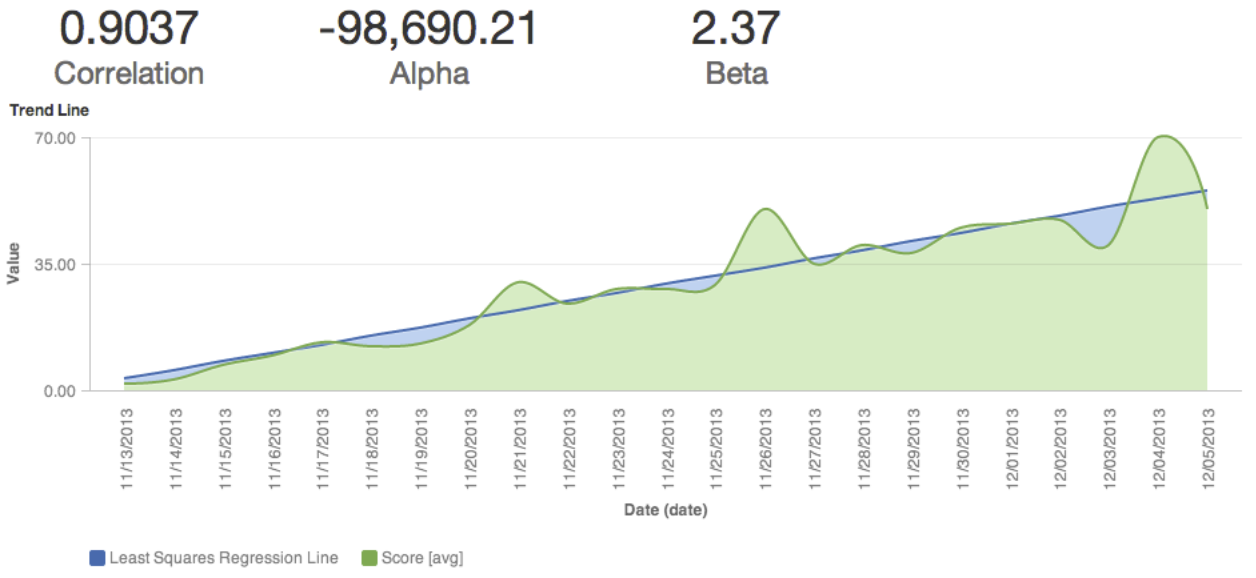
This linear regression line may not show as a continuous straight line if you are missing values for x in your sample. You can fix this issue by generating null y values when x values do not exist, and making any necessary "if null" protections within the underlying metrics. See IFNULL in our Documentation.
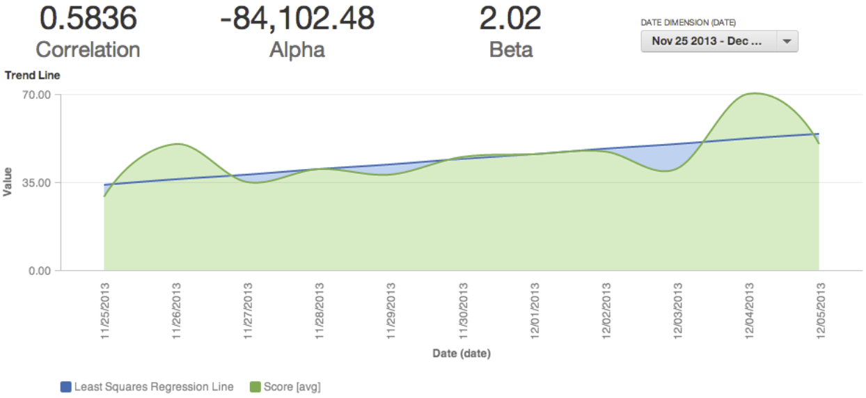
Try adding a filter
Optionally, you may add a filter on x values to adjust on the fly, which enables discovery of how the correlation coefficient and your linear regression line change for different partitions of your data:
There are potential applications to expand this linear regression model to even complex predictive reporting such as polynomial regression and risk exposure. By nesting MAQL metrics, you can create complex statistical expressions with little of the complexity you'd expect from a data query language.